Land Slippage

In the summer of 2017 FlyThru were tasked to conduct a LiDAR survey to examine a large sloping area on the bank of a river. The area has been suspected to be liable to subsidence and was covered in natural vegetation. Although instructed to perform LiDAR surveys of the area, a photogrammetry mission was also undertaken to colourise the collected LiDAR data.
When using LiDAR to accurately survey an area there are two main factors to consider. Firstly, it must be determined if the LiDAR sensor can sufficiently penetrate the vegetation, and secondly the best processing methodology for producing the most accurate DSM and DTM must be identified.
Below are examples that demonstrate FlyThru LiDAR vegetation penetration and processing expertise:
Firstly, the ability of the FlyThru’s LiDAR system to penetrate dense vegetation.

This image highlights the type of vegetation present on much of the surveyed bank. Within the center of the image you can see a dense area of ‘rhubarb-like’ vegetation. The tightly packed plants with large broad leaves make it challenging surveying terrain for LiDAR to penetrate the surface to collect ground points.
The image below shows the classified LiDAR point cloud with brown representing ground points and black representing non-ground points. With aerial LiDAR alternatives, it is unlikely that any ground point penetration would occur with such dense vegetation. This image, however, demonstrates that FlyThru’s LiDAR system is able to collect ground points through almost impenetrable vegetation.

The following image shows only ground points, proving that even through dense vegetation there is still an adequate acquisition of ground points for terrain to be mapped and movement of earth be monitored.

As vegetation penetration is sufficient, we must next consider data processing options.
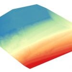
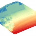
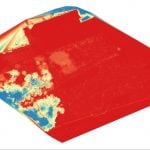
FlyThru can produce outputs representing the difference in elevation between a DTM and DSM, showing where vegetation was much higher than the ground. This allows for a better understanding and visualisation of the area being analysed, for example by allowing drainage channels within earthworks or a peat bog to be located that are hidden below vegetation.
This visualisation can be achieved through several methods, and is demonstrated below where a DSM, DTM, difference between these layers and hillshade 3D representation are shown.
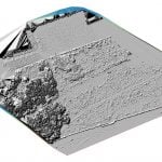
This final image is a hillshade raster created from the difference between the DSM and DTM models. by visualising as a hillshade it is possible to visualise the elevation of the vegetation about the DTM.
Case Study Output Accuracy
The LiDAR system uses a survey base station to provide live real time kinematic (RTK) correction over short distances to the LiDAR sensor. This leads to an overall relative accuracy of 20 mm and a true geo-accuracy of 50 mm – that is to say that the model is internally consistent to an accuracy of 20 mm within each frame of LiDAR data, however the overall dataset contains a small additional shift in any direction (due to GPS accuracy) giving a total accuracy of 50 mm.